How to Calculate Instantaneous Rate of Change

In many scenarios, understanding the exact rate at which things change at a specific moment can be crucial. From the speed of a car at the exact second you tap the brakes to the rate a hot cup of coffee cools, knowing the instantaneous rate of change helps us make sense of dynamic processes. Mathematically, this concept is vital in fields such as physics, engineering, and economics. Normally, it is calculated using calculus, specifically by finding the derivative of a function. Let’s demystify this concept and learn how anyone can approach finding the instantaneous rate of change, step by step.

Using the Definition of the Derivative

To understand the instantaneous rate of change, we begin by delving into the basic principles of calculus. The definition of the derivative offers a direct method for finding that precise rate at which a function changes at any given point.

Detailed Steps:

1. Write down the function for which you wish to find the instantaneous rate of change.

2. Identify the specific point at which you need to find the rate of change. Let’s call this point a.

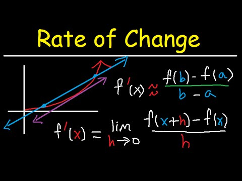
3. Apply the definition of the derivative, which is the limit of the average rate of change as the interval approaches zero:

   [ f’(a)= lim_{{x to a}} frac{f(x) – f(a)}{x – a} ]

4. Substitute the function and the point a into the formula.

5. Simplify the expression.

6. Take the limit as x approaches a.

7. The result you obtain is the instantaneous rate of change of the function at the point a.

Summary:

This method provides a solid foundation for understanding and calculating the instantaneous rate of change, directly derived from calculus principles. While this approach can be seen as the most “mathematically pure,” it may be intimidating for those who are not familiar with calculus and limits.

Graphical Interpretation

For a more visual understanding, the instantaneous rate of change can also be seen by looking at a graph of the function you are interested in.

Detailed Steps:

1. Plot the function on a graph.

2. Locate the point at which you want to determine the rate of change.

3. Draw a tangent line to the curve at this point.

4. Find two points on this tangent line that are close to the point of tangency.

5. Use these two points to calculate the slope of the tangent line (rise over run).

6. The slope of this tangent line is the instantaneous rate of change at the chosen point.

Summary:

This intuitive approach offers a visual way to estimate the instantaneous rate of change without explicitly using calculus. However, it may lack precision, especially if the curve is complex or if the tangent line is hard to draw accurately.

Numerical Approximation

Sometimes, an approximation of the instantaneous rate of change is sufficient, especially when a function is not easily differentiable or when you have discrete data points.

Detailed Steps:

1. Choose two points that are very close to the point of interest on the function.

2. Calculate the average rate of change between these points:

   [ frac{f(x_2) – f(x_1)}{x_2 – x_1} ]

3. The closer these points are to each other, the better the approximation of the instantaneous rate of change.

4. Repeat the calculation with points increasingly closer together to improve the estimate.

Summary:

This method is particularly useful for dealing with emprical data or when you need a quick estimate. The downside is that it is only an approximation and accuracy can vary greatly depending on your choice of points.

Increment and Difference Quotient

Another numerical method involves using the difference quotient to estimate the derivative.

Detailed Steps:

1. Choose a small increment, h, which will approach zero.

2. Calculate the difference quotient:

   [ frac{f(a+h) – f(a)}{h} ]

3. The smaller the increment h, the closer the quotient will be to the instantaneous rate of change at point a.

4. Evaluate the quotient for progressively smaller values of h.

Summary:

This technique is a step towards using the limits concept in calculus but remains accessible to those without an extensive math background. It does require some trial and error to find a sufficiently small h for a good approximation.

Calculator Methods

Modern calculators, especially graphing calculators, come equipped with functions to find derivatives, which can be used to calculate instantaneous rates of change.

Detailed Steps:

1. Enter your function into the calculator.

2. Navigate to the derivative function (this varies by calculator).

3. Input the specific point a.

4. The calculator will compute the rate of change for you.

Summary:

This method is very user-friendly and provides an accurate result quickly, assuming the calculator is programmed correctly. The downside is that it may not help in understanding the underlying principles of the calculation.

Spreadsheet Software

Programs like Microsoft Excel, Google Sheets, or other spreadsheet tools can be used to calculate instantaneous rates of change by creating a table of values and using built-in formulas.

Detailed Steps:

1. Input the function into the spreadsheet as a formula.

2. Generate a table of values, including f(a) and values for f(a+h) where h is very small.

3. Use the spreadsheet’s built-in functions to calculate the derivative or apply the difference quotient.

4. Interpret the results from the table to approximate the instantaneous rate of change.

Summary:

Spreadsheets provide a more tangible way to visualize the process of calculating rates of change. They are especially useful for handling large datasets but can be less intuitive for one-off calculations.

Algebraic Simplification

In cases where the function has a simple algebraic form, finding the derivative can often be done by hand through algebraic manipulation.

Detailed Steps:

1. Express the function in its simplest form, if possible.

2. Use known derivative rules (such as the power rule) to differentiate the function.

3. Plug in the point of interest a into the derivative to find the instantaneous rate of change.

Summary:

This approach reinforces mathematical concepts and demonstrates a clear, step-by-step calculation process. However, it assumes some knowledge of differentiation rules and algebra.

With these methods, one can approach the problem of calculating the instantaneous rate of change from different angles, each suited to the individual’s preference, understanding, and available tools.

Conclusion

The instantaneous rate of change is a vital concept that reveals how quickly things move or shift at a specific point in time. By using methods from calculus, graph analysis, numerical approximations, and even technology, anyone can approach this concept and understand the dynamics of change in various contexts. Whether you’re analyzing data, creating models, or simply satisfying curiosity, mastering this calculation broadens your analytical toolkit.

FAQs

1. What is the difference between average and instantaneous rates of change?
   The average rate of change measures how much a function changes over an interval, while the instantaneous rate of change measures how much the function changes at a particular point, namely, at an instant.

2. Why is calculus important for determining the instantaneous rate of change?
   Calculus provides the tools, specifically derivatives, to measure and analyze rates of change at any given point on a function, which is something algebra alone cannot accomplish.

3. Can I calculate the instantaneous rate of change without using calculus?
   Yes, there are numerical and graphical methods to approximate the instantaneous rate of change, although they might not provide the same precision as calculus-based methods.